Python使用ReportLab画图

q66262

　　本文主要介绍如何借助ReportLab画图。
　　首先看一下经典的hello word：

#!/usr/bin/env python
from reportlab.graphics.shapes import Drawing, String
from reportlab.graphics import renderPDF
d = Drawing(100, 100)
s = String(50, 50, 'Hello, world!', textAnchor='middle')
d.add(s)
renderPDF.drawToFile(d, 'hello.pdf', 'A simple PDF file')


　　运行后可发现当前路径下多了一个hello.pdf，在中间写着hello world
　　

　　下面用其根据数据画图，代码如下：

#!/usr/bin/env python
from reportlab.lib import colors
from reportlab.graphics.shapes import *
from reportlab.graphics import renderPDF
data = [
#    Year  Month  Predicted  High  Low
(2007,  8,    113.2,     114.2, 112.2),
(2007,  9,    112.8,     115.8, 109.8),
(2007, 10,    111.0,     116.0, 106.0),
(2007, 11,    109.8,     116.8, 102.8),
(2007, 12,    107.3,     115.3,  99.3),
(2008,  1,    105.2,     114.2,  96.2),
(2008,  2,    104.1,     114.1,  94.1),
(2008,  3,     99.9,     110.9,  88.9),
(2008,  4,     94.8,     106.8,  82.8),
(2008,  5,     91.2,     104.2,  78.2),
]
drawing = Drawing(200, 150)
pred = [row[2]-40 for row in data]
high = [row[3]-40 for row in data]
low = [row[4]-40 for row in data]
times = [200*((row[0] + row[1]/12.0) - 2007)-110 for row in data]
drawing.add(PolyLine(zip(times, pred), strokeColor=colors.blue))
drawing.add(PolyLine(zip(times, high), strokeColor=colors.red))
drawing.add(PolyLine(zip(times, low),  strokeColor=colors.green))
drawing.add(String(65, 115, 'Sunspots', fontSize=18, fillColor=colors.red))
renderPDF.drawToFile(drawing, 'report1.pdf', 'Sunspots')


运行结果如下：

　　

　　然后根据网页上的数据进行画图：
　　代码如下：

from urllib import urlopen
from reportlab.graphics.shapes import *
from reportlab.graphics.charts.lineplots import LinePlot
from reportlab.graphics.charts.textlabels import Label
from reportlab.graphics import renderPDF
URL = 'http://www.swpc.noaa.gov/ftpdir/weekly/Predict.txt'
COMMENT_CHARS = '#:'

drawing = Drawing(400, 200)
data = []
for line in urlopen(URL).readlines():
if not line.isspace() and not line[0] in COMMENT_CHARS:
data.append([float(n) for n in line.split()])
pred = [row[2] for row in data]
high = [row[3] for row in data]
low = [row[4] for row in data]
times = [row[0] + row[1]/12.0 for row in data]
lp = LinePlot()
lp.x = 50
lp.y = 50
lp.height = 125
lp.width = 300
lp.data = [zip(times, pred), zip(times, high), zip(times, low)]
lp.lines[0].strokeColor = colors.blue
lp.lines[1].strokeColor = colors.red
lp.lines[2].strokeColor = colors.green
drawing.add(lp)
drawing.add(String(250, 150, 'Sunspots',
fontSize=14, fillColor=colors.red))

renderPDF.drawToFile(drawing, 'report2.pdf', 'Sunspots')其中http://www.swpc.noaa.gov/ftpdir/weekly/Predict.txt中的数据如下所示：
:Predicted_Sunspot_Numbers_and_Radio_Flux: Predict.txt
:Created: 2013 Nov 04 0600 UTC
# Prepared by the U.S. Dept. of Commerce, NOAA, Space Weather Prediction Center (SWPC).
# Please send comments and suggestions to swpc.webmaster@noaa.gov
#
# Sunspot Number: S.I.D.C. Brussels International Sunspot Number.
# 10.7cm Radio Flux value: Penticton, B.C. Canada.
# Predicted values are based on the consensus of the Solar Cycle 24 Prediction Panel.
#
# See the README3 file for further information.
#
# Missing or not applicable data:  -1
#
#         Predicted Sunspot Number And Radio Flux Values
#                     With Expected Ranges
#
#         -----Sunspot Number------  ----10.7 cm Radio Flux----
# YR MO   PREDICTED    HIGH    LOW   PREDICTED    HIGH    LOW
#--------------------------------------------------------------
2013 05        60.3    61.3    59.3      117.8   118.8   116.8
2013 06        63.3    65.3    61.3      119.8   120.8   118.8
2013 07        66.2    69.2    63.2      121.5   123.5   119.5
2013 08        69.2    74.2    64.2      123.3   126.3   120.3
2013 09        72.3    77.3    67.3      125.8   129.8   121.8
2013 10        73.9    79.9    67.9      127.3   131.3   123.3
2013 11        74.5    81.5    67.5      127.8   132.8   122.8
2013 12        75.9    82.9    68.9      128.9   134.9   122.9
2014 01        78.1    86.1    70.1      130.6   137.6   123.6
2014 02        79.6    88.6    70.6      132.0   140.0   124.0
2014 03        81.8    90.8    72.8      133.8   141.8   125.8
2014 04        83.1    93.1    73.1      134.8   143.8   125.8
2014 05        82.2    92.2    72.2      134.1   143.1   125.1
2014 06        81.4    91.4    71.4      133.5   142.5   124.5
2014 07        80.2    90.2    70.2      132.3   141.3   123.3
2014 08        78.9    88.9    68.9      131.2   140.2   122.2
2014 09        77.6    87.6    67.6      129.9   138.9   120.9
2014 10        76.2    86.2    66.2      128.7   137.7   119.7
2014 11        74.8    84.8    64.8      127.4   136.4   118.4
2014 12        73.3    83.3    63.3      126.0   135.0   117.0
2015 01        71.8    81.8    61.8      124.6   133.6   115.6
2015 02        70.2    80.2    60.2      123.2   132.2   114.2
2015 03        68.7    78.7    58.7      121.7   130.7   112.7
2015 04        67.0    77.0    57.0      120.2   129.2   111.2
2015 05        65.4    75.4    55.4      118.7   127.7   109.7
2015 06        63.8    73.8    53.8      117.2   126.2   108.2
2015 07        62.1    72.1    52.1      115.7   124.7   106.7
2015 08        60.4    70.4    50.4      114.1   123.1   105.1
2015 09        58.7    68.7    48.7      112.6   121.6   103.6
2015 10        57.0    67.0    47.0      111.0   120.0   102.0
2015 11        55.3    65.3    45.3      109.5   118.5   100.5
2015 12        53.6    63.6    43.6      107.9   116.9    98.9
2016 01        51.9    61.9    41.9      106.3   115.3    97.3
2016 02        50.2    60.2    40.2      104.8   113.8    95.8
2016 03        48.5    58.5    38.5      103.2   112.2    94.2
2016 04        46.9    56.9    36.9      101.7   110.7    92.7
2016 05        45.2    55.2    35.2      100.2   109.2    91.2
2016 06        43.6    53.6    33.6       98.7   107.7    89.7
2016 07        42.0    52.0    32.0       97.2   106.2    88.2
2016 08        40.4    50.4    30.4       95.8   104.8    86.8
2016 09        38.8    48.8    28.8       94.3   103.3    85.3
2016 10        37.3    47.3    27.3       92.9   101.9    83.9
2016 11        35.7    45.7    25.7       91.5   100.5    82.5
2016 12        34.3    44.3    24.3       90.2    99.2    81.2
2017 01        32.8    42.8    22.8       88.8    97.8    79.8
2017 02        31.4    41.4    21.4       87.5    96.5    78.5
2017 03        30.0    40.0    20.0       86.3    95.3    77.3
2017 04        28.7    38.7    18.7       85.0    94.0    76.0
2017 05        27.4    37.4    17.4       83.8    92.8    74.8
2017 06        26.1    36.1    16.1       82.6    91.6    73.6
2017 07        24.9    34.9    14.9       81.5    90.5    72.5
2017 08        23.7    33.7    13.7       80.4    89.4    71.4
2017 09        22.5    32.5    12.5       79.3    88.3    70.3
2017 10        21.4    31.4    11.4       78.3    87.3    69.3
2017 11        20.3    30.3    10.3       77.3    86.3    68.3
2017 12        19.2    29.2     9.2       76.4    85.4    67.4
2018 01        18.2    28.2     8.2       75.4    84.4    66.4
2018 02        17.2    27.2     7.2       74.5    83.5    65.5
2018 03        16.3    26.3     6.3       73.7    82.7    64.7
2018 04        15.4    25.4     5.4       72.8    81.8    63.8
2018 05        14.5    24.5     4.5       72.1    81.1    63.1
2018 06        13.7    23.7     3.7       71.3    80.3    62.3
2018 07        12.9    22.9     2.9       70.6    79.6    61.6
2018 08        12.2    22.2     2.2       69.9    78.9    60.9
2018 09        11.5    21.5     1.5       69.2    78.2    60.2
2018 10        10.8    20.8     0.8       68.6    77.6    60.0
2018 11        10.1    20.1     0.1       68.0    77.0    60.0
2018 12         9.5    19.5     0.0       67.4    76.4    60.0
2019 01         8.9    18.9     0.0       66.9    75.9    60.0
2019 02         8.3    18.3     0.0       66.3    75.3    60.0
2019 03         7.8    17.8     0.0       65.9    74.9    60.0
2019 04         7.3    17.3     0.0       65.4    74.4    60.0
2019 05         6.8    16.8     0.0       65.0    74.0    60.0
2019 06         6.4    16.4     0.0       64.5    73.5    60.0
2019 07         5.9    15.9     0.0       64.1    73.1    60.0
2019 08         5.5    15.5     0.0       63.8    72.8    60.0
2019 09         5.1    15.1     0.0       63.4    72.4    60.0
2019 10         4.8    14.8     0.0       63.1    72.1    60.0
2019 11         4.4    14.4     0.0       62.8    71.8    60.0
2019 12         4.1    14.1     0.0       62.5    71.5    60.0

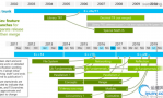
运行结果如下：