Practicing Machine Learning Techniques in R with MLR Package

lixiaolong

Introduction
　　In R, we often use multiple packages for doing various machine learning tasks. For example: we impute missing value using one package, then build a model with another and finally evaluate their performance using a third package.
　　The problem is, every package has a set of specific parameters. While working with many packages, we end up spending a lot of time to figure out which parameters are important. Don’t you think?
　　To solve this problem, I researched and came across a R package named MLR, which is absolutely incredible at performing machine learning tasks. This package includes all of the ML algorithms which we use frequently.
　　In this tutorial, I’ve taken up a classification problem and tried improving its accuracy using machine learning. I haven’t explained the ML algorithms (theoretically) but focus is kept on their implementation. By the end of this article, you are expected to become proficient at implementing several ML algorithms in R. But, only if you practice alongside.
　　Note: This article is meant only for beginners and early starters with Machine Learning in R. Basic statistic knowledge is required.

Table of Content

• Getting Data
  
• Exploring Data
  
• Missing Value Imputation
  
• Feature Engineering
  
  
  
  • Outlier Removal by Capping
    
  • New Features
    
  
  
• Machine Learning
  
  
  
  • Feature Importance
    
  • QDA
    
  • Logistic Regression
    
    
    
    • Cross Validation
      
    
    
  • Decision Tree
    
    
    
    • Cross Validation
      
    • Parameter Tuning using Grid Search
      
    
    
  • Random Forest
    
  • SVM
    
  • GBM (Gradient Boosting)
    
    
    
    • Cross Validation
      
    • Parameter Tuning using Random Search (Faster)
      
    
    
  • XGBoost (Extreme Gradient Boosting)
    
  • Feature Selection
    
  
  

Machine Learning with MLR Package
　　Until now, R didn’t have any package / library similar to Scikit-Learn from Python, wherein you could get all the functions required to do machine learning. But, since February 2016, R users have got mlr package using which they can perform most of their ML tasks.
　　Let’s now understand the basic concept of how this package works. If you get it right here, understanding the whole package would be a mere cakewalk.
　　The entire structure of this package relies on this premise:
　　Create a Task. Make a Learner. Train Them.
　　Creating a task means loading data in the package. Making a learner means choosing an algorithm ( learner) which learns from task (or data). Finally, train them.
　　MLR package has several algorithms in its bouquet. These algorithms have been categorized into regression, classification, clustering, survival, multiclassification and cost sensitive classification. Let’s look at some of the available algorithms for classification problems:
　　> listLearners("classif")[c("class","package")]
  class                           package
1 classif.avNNet                   nnet
2 classif.bartMachine            bartMachine
3 classif.binomial                 stats
4 classif.boosting               adabag,rpart
5 classif.cforest                  party
6 classif.ctree                    party
7 classif.extraTrees             extraTrees
8 classif.knn                      class
9 classif.lda                      MASS
10 classif.logreg                  stats
11 classif.lvq1                    class
12 classif.multinom                 nnet
13 classif.neuralnet             neuralnet
14 classif.nnet                     nnet
15 classif.plsdaCaret              caret
16 classif.probit                  stats
17 classif.qda                      MASS
18 classif.randomForest         randomForest
19 classif.randomForestSRC      randomForestSRC
20 classif.randomForestSRCSyn   randomForestSRC
21 classif.rpart                    rpart
22 classif.xgboost                 xgboost
　　And, there are many more. Let’s start working now!
1. Getting Data
　　For this tutorial, I’ve taken up one of the popular ML problem from DataHack: Download Data.
　　After you’ve downloaded the data, let’s quickly get done with initial commands such as setting the working directory and loading data.
　　> path <- "~/Data/Playground/MLR_Package"
> setwd(path)
　　#load libraries and data
> install.packages("mlr")
> library(mlr)
> train <- read.csv("train_loan.csv", na.strings = c(""," ",NA))
> test <- read.csv("test_Y3wMUE5.csv", na.strings = c(""," ",NA))
2. Exploring Data
　　Once the data is loaded, you can access it using:
　　> summarizeColumns(train)
　　name              type    na    mean           disp      median     mad    min   max   nlevs
LoanAmount       integer  22   146.4121622  85.5873252   128.0   47.4432    9    700    0
Loan_Amount_Term integer  14   342.0000000  65.1204099   360.0    0.0000   12    480    0
Credit_History   integer  50   0.8421986    0.3648783     1.0     0.0000   0      1     0
Property_Area    factor   0      NA         0.6205212     NA        NA    179    233    3
Loan_Status      factor   0      NA         0.3127036     NA        NA    192    422    2
　　This functions gives a much comprehensive view of the data set as compared to base str()function. Shown above are the last 5 rows of the result. Similarly you can do for test data also:
　　> summarizeColumns(test)
　　From these outputs, we can make the following inferences:

• In the data, we have 12 variables, out of which Loan_Status is the dependent variable and rest are independent variables.
  
• Train data has 614 observations. Test data has 367 observations.
  
• In train and test data, 6 variables have missing values (can be seen in na column).
  
• ApplicantIncome and Coapplicant Income are highly skewed variables. How do we know that ? Look at their min, max and median value. We’ll have to normalize these variables.
  
• LoanAmount, ApplicantIncome and CoapplicantIncome has outlier values, which should be treated.
  
• Credit_History is an integer type variable. But, being binary in nature, we should convert it to factor.
  

　　Also, you can check the presence of skewness in variables mentioned above using a simple histogram.
　　> hist(train$ApplicantIncome, breaks = 300, main = "Applicant Income Chart",xlab = "ApplicantIncome")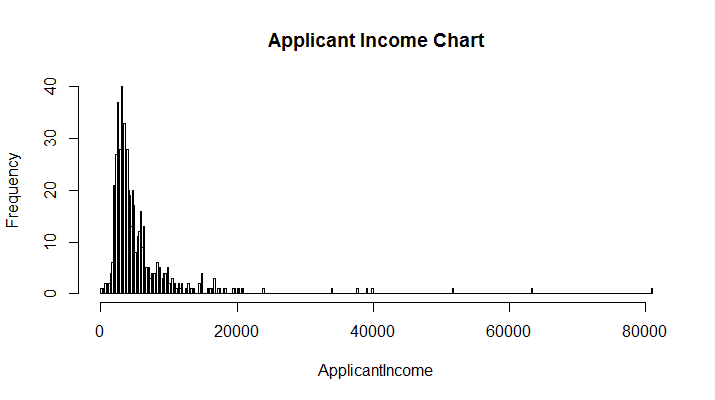
　　> hist(train$CoapplicantIncome, breaks = 100,main = "Coapplicant Income Chart",xlab = "CoapplicantIncome")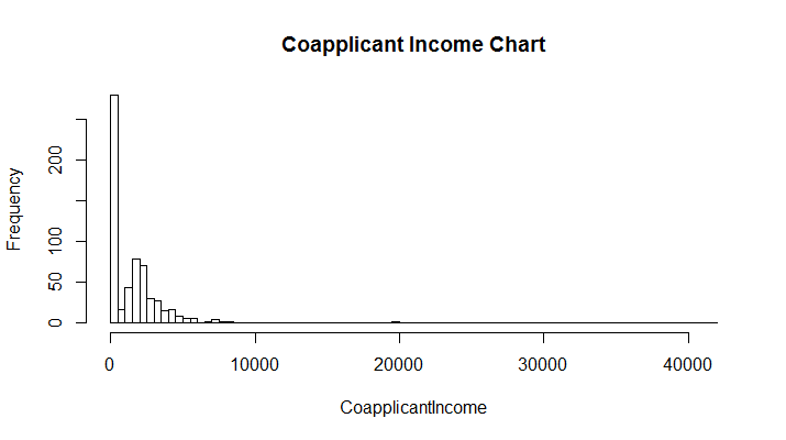
　　As you can see in charts above, skewness is nothing but concentration of majority of data on one side of the chart. What we see is a right skewed graph. To visualize outliers, we can use a boxplot:
　　> boxplot(train$ApplicantIncome)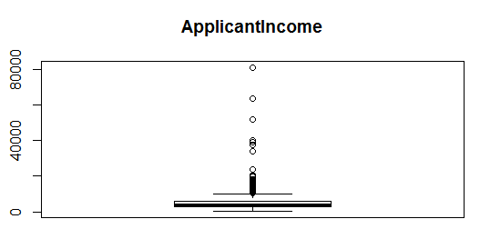
　　Similarly, you can create a boxplot for CoapplicantIncome and LoanAmount as well.
　　Let’s change the class of Credit_History to factor. Remember, the class factor is always used for categorical variables.
　　> train$Credit_History <- as.factor(train$Credit_History)
> test$Credit_History <- as.factor(test$Credit_History)
　　To check the changes, you can do:
　　> class(train$Credit_History)
[1] "factor"
　　You can further scrutinize the data using:
　　> summary(train)
> summary(test)
　　We find that the variable Dependents has a level 3+ which shall be treated too. It’s quite simple to modify the name levels in a factor variable. It can be done as:
　　#rename level of Dependents
> levels(train$Dependents)[4] <- "3"
> levels(test$Dependents)[4] <- "3"
3. Missing Value Imputation
　　Not just beginners, even good R analyst struggle with missing value imputation. MLR package offers a nice and convenient way to impute missing value using multiple methods. After we are done with much needed modifications in data, let’s impute missing values.
　　In our case, we’ll use basic mean and mode imputation to impute data. You can also use any ML algorithm to impute these values, but that comes at the cost of computation.
　　#impute missing values by mean and mode
> imp <- impute(train, classes = list(factor = imputeMode(), integer = imputeMean()), dummy.classes = c("integer","factor"), dummy.type = "numeric")
> imp1 <- impute(test, classes = list(factor = imputeMode(), integer = imputeMean()), dummy.classes = c("integer","factor"), dummy.type = "numeric")
　　This function is convenient because you don’t have to specify each variable name to impute. It selects variables on the basis of their classes. It also creates new dummy variables for missing values. Sometimes, these (dummy) features contain a trend which can be captured using this function.dummy.classes says for which classes should I create a dummy variable. dummy.type says what should be the class of new dummy variables.
　　$data attribute of imp function contains the imputed data.
　　> imp_train <- imp$data
> imp_test <- imp1$data
　　Now, we have the complete data. You can check the new variables using:
　　>summarizeColumns(imp_train)
>summarizeColumns(imp_test)
　　Did you notice a disparity among both data sets? No ? See again. The answer is Married.dummyvariable exists only in imp_train and not in imp_test. Therefore, we’ll have to remove it before modeling stage.
　　Optional: You might be excited or curious to try out imputing missing values using a ML algorithm. In fact, there are some algorithms which don’t require you to impute missing values. You can simply supply them missing data. They take care of missing values on their own. Let’s see which algorithms are they:
　　> listLearners("classif", check.packages = TRUE, properties = "missings")[c("class","package")]
class                           package
1 classif.bartMachine          bartMachine
2 classif.boosting            adabag,rpart
3 classif.cforest                party
4 classif.ctree                  party
5 classif.gbm                     gbm
6 classif.naiveBayes             e1071
7 classif.randomForestSRC   randomForestSRC
8 classif.rpart                  rpart
　　However, it is always advisable to treat missing values separately. Let’s see how can you treat missing value using rpart:
　　> rpart_imp <- impute(train, target = "Loan_Status",
classes = list(numeric = imputeLearner(makeLearner("regr.rpart")),
factor = imputeLearner(makeLearner("classif.rpart"))),
dummy.classes = c("numeric","factor"),
dummy.type = "numeric")
4. Feature Engineering
　　Feature Engineering is the most interesting part of predictive modeling. So, feature engineering has two aspects: Feature Transformation and Feature Creation. We’ll try to work on both the aspects here.
　　At first, let’s remove outliers from variables like ApplicantIncome, CoapplicantIncome, LoanAmount. There are many techniques to remove outliers. Here, we’ll cap all the large values in these variables and set them to a threshold value as shown below:
　　#for train data set
> cd <- capLargeValues(imp_train, target = "Loan_Status",cols = c("ApplicantIncome"),threshold = 40000)
> cd <- capLargeValues(cd, target = "Loan_Status",cols = c("CoapplicantIncome"),threshold = 21000)
> cd <- capLargeValues(cd, target = "Loan_Status",cols = c("LoanAmount"),threshold = 520)
　　#rename the train data as cd_train
> cd_train <- cd
　　#add a dummy Loan_Status column in test data
> imp_test$Loan_Status <- sample(0:1,size = 367,replace = T)
　　> cde <- capLargeValues(imp_test, target = "Loan_Status",cols = c("ApplicantIncome"),threshold = 33000)
> cde <- capLargeValues(cde, target = "Loan_Status",cols = c("CoapplicantIncome"),threshold = 16000)
> cde <- capLargeValues(cde, target = "Loan_Status",cols = c("LoanAmount"),threshold = 470)
　　#renaming test data
> cd_test <- cde
　　I’ve chosen the threshold value with my discretion, after analyzing the variable distribution. To check the effects, you can do summary(cd_train$ApplicantIncome) and see that the maximum value is capped at 33000.
　　In both data sets, we see that all dummy variables are numeric in nature. Being binary in form, they should be categorical. Let’s convert their classes to factor. This time, we’ll use simple for and ifloops.
　　#convert numeric to factor - train
> for (f in names(cd_train[, c(14:20)])) {
if( class(cd_train[, c(14:20)] [[f]]) == "numeric"){
levels <- unique(cd_train[, c(14:20)][[f]])
cd_train[, c(14:20)][[f]] <- as.factor(factor(cd_train[, c(14:20)][[f]], levels = levels))
}
}
　　#convert numeric to factor - test
> for (f in names(cd_test[, c(13:18)])) {
if( class(cd_test[, c(13:18)] [[f]]) == "numeric"){
levels <- unique(cd_test[, c(13:18)][[f]])
cd_test[, c(13:18)][[f]] <- as.factor(factor(cd_test[, c(13:18)][[f]], levels = levels))
}
}
　　These loops say – ‘for every column name which falls column number 14 to 20 of cd_train / cd_test data frame, if the class of those variables in numeric, take out the unique value from those columns as levels and convert them into a factor (categorical) variables.
　　Let’s create some new features now.
　　#Total_Income
> cd_train$Total_Income <- cd_train$ApplicantIncome + cd_train$CoapplicantIncome
> cd_test$Total_Income <- cd_test$ApplicantIncome + cd_test$CoapplicantIncome
　　#Income by loan
> cd_train$Income_by_loan <- cd_train$Total_Income/cd_train$LoanAmount
> cd_test$Income_by_loan <- cd_test$Total_Income/cd_test$LoanAmount
　　#change variable class
> cd_train$Loan_Amount_Term <- as.numeric(cd_train$Loan_Amount_Term)
> cd_test$Loan_Amount_Term <- as.numeric(cd_test$Loan_Amount_Term)
　　#Loan amount by term
> cd_train$Loan_amount_by_term <- cd_train$LoanAmount/cd_train$Loan_Amount_Term
> cd_test$Loan_amount_by_term <- cd_test$LoanAmount/cd_test$Loan_Amount_Term
　　While creating new features(if they are numeric), we must check their correlation with existing variables as there are high chances often. Let’s see if our new variables too happens to be correlated:
　　#splitting the data based on class
> az <- split(names(cd_train), sapply(cd_train, function(x){ class(x)}))
　　#creating a data frame of numeric variables
> xs <- cd_train[az$numeric]
　　#check correlation
> cor(xs)
　　As we see, there exists a very high correlation of Total_Income with ApplicantIncome. It means that the new variable isn’t providing any new information. Thus, this variable is not helpful for modeling data.
　　Now we can remove the variable.
　　> cd_train$Total_Income <- NULL
> cd_test$Total_Income <- NULL
　　There is still enough potential left to create new variables. Before proceeding, I want you to think deeper on this problem and try creating newer variables. After doing so much modifications in data, let’s check the data again:
　　> summarizeColumns(cd_train)
> summarizeColumns(cd_test)
5. Machine Learning
　　Until here, we’ve performed all the important transformation steps except normalizing the skewed variables. That will be done after we create the task.
　　As explained in the beginning, for mlr, a task is nothing but the data set on which a learner learns. Since, it’s a classification problem, we’ll create a classification task. So, the task type solely depends on type of problem at hand.
　　#create a task
> trainTask <- makeClassifTask(data = cd_train,target = "Loan_Status")
> testTask <- makeClassifTask(data = cd_test, target = "Loan_Status")
　　Let’s check trainTask
　　> trainTask
Supervised task: cd_train
Type: classif
Target: Loan_Status
Observations: 614
Features:
numerics factors ordered
13         8       0
Missings: FALSE
Has weights: FALSE
Has blocking: FALSE
Classes: 2
N   Y
192 422
Positive class: N
　　As you can see, it provides a description of cd_train data. However, an evident problem is that it is considering positive class as N, whereas it should be Y. Let’s modify it:
　　> trainTask <- makeClassifTask(data = cd_train,target = "Loan_Status", positive = "Y")
　　For a deeper view, you can check your task data using str(getTaskData(trainTask)).
　　Now, we will normalize the data. For this step, we’ll use normalizeFeatures function from mlr package. By default, this packages normalizes all the numeric features in the data. Thankfully, only 3 variables which we have to normalize are numeric, rest of the variables have classes other than numeric.
　　#normalize the variables
> trainTask <- normalizeFeatures(trainTask,method = "standardize")
> testTask <- normalizeFeatures(testTask,method = "standardize")
　　Before we start applying algorithms, we should remove the variables which are not required.
　　> trainTask <- dropFeatures(task = trainTask,features = c("Loan_ID","Married.dummy"))
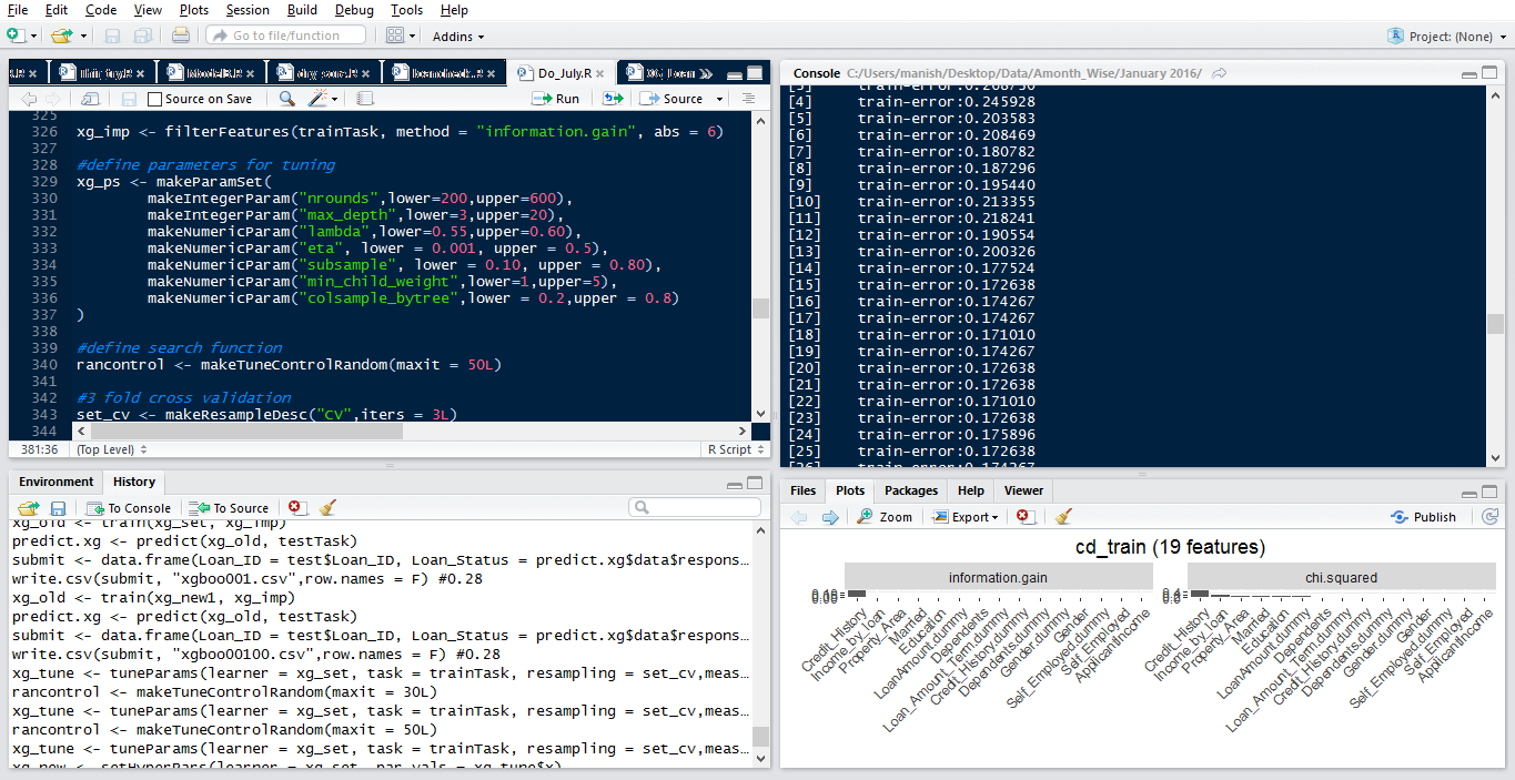
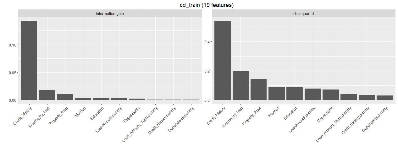
　　MLR package has an in built function which returns the important variables from data. Let’s see which variables are important. Later, we can use this knowledge to subset out input predictors for model improvement. While running this code, R might prompt you to install ‘FSelector’ package, which you should do.
　　#Feature importance
> im_feat <- generateFilterValuesData(trainTask, method = c("information.gain","chi.squared"))
> plotFilterValues(im_feat,n.show = 20)

　　#to launch its shiny application
> plotFilterValuesGGVIS(im_feat)
　　If you are still wondering about information.gain, let me provide a simple explanation. Information gain is generally used in context with decision trees. Every node split in a decision tree is based on information gain. In general, it tries to find out variables which carries the maximum information using which the target class is easier to predict.
　　Let’s start modeling now. I won’t explain these algorithms in detail but I’ve provided links to helpful resources. We’ll take up simpler algorithms at first and end this tutorial with the complexed ones.
　　With MLR, we can choose & set algorithms using makeLearner. This learner will train on trainTaskand try to make predictions on testTask.
　　1. Quadratic Discriminant Analysis (QDA).
　　In general, qda is a parametric algorithm. Parametric means that it makes certain assumptions about data. If the data is actually found to follow the assumptions, such algorithms sometime outperform several non-parametric algorithms. Read More.
　　#load qda
> qda.learner <- makeLearner("classif.qda", predict.type = "response")
　　#train model
> qmodel <- train(qda.learner, trainTask)
　　#predict on test data
> qpredict <- predict(qmodel, testTask)
　　#create submission file
> submit <- data.frame(Loan_ID = test$Loan_ID, Loan_Status = qpredict$data$response)
> write.csv(submit, "submit1.csv",row.names = F)
　　Upload this submission file and check your leaderboard rank (wouldn’t be good). Our accuracy is ~ 71.5%. I understand, this submission might not put you among the top on leaderboard, but there’s along way to go. So, let’s proceed.
　　2. Logistic Regression
　　This time, let’s also check cross validation accuracy. Higher CV accuracy determines that our model does not suffer from high variance and generalizes well on unseen data.
　　#logistic regression
> logistic.learner <- makeLearner("classif.logreg",predict.type = "response")
　　#cross validation (cv) accuracy
> cv.logistic <- crossval(learner = logistic.learner,task = trainTask,iters = 3,stratify = TRUE,measures = acc,show.info = F)
　　Similarly, you can perform CV for any learner. Isn’t it incredibly easy? So, I’ve used stratified sampling with 3 fold CV. I’d always recommend you to use stratified sampling in classification problems since it maintains the proportion of target class in n folds. We can check CV accuracy by:
　　#cross validation accuracy
> cv.logistic$aggr
acc.test.mean
0.7947553

　　This is the average accuracy calculated on 5 folds. To see, respective accuracy each fold, we can do this:
　　> cv.logistic$measures.test
  iter    acc
1  1    0.8439024
2  2    0.7707317
3  3    0.7598039
　　Now, we’ll train the model and check the prediction accuracy on test data.
　　#train model
> fmodel <- train(logistic.learner,trainTask)
> getLearnerModel(fmodel)
　　#predict on test data
> fpmodel <- predict(fmodel, testTask)
　　#create submission file
> submit <- data.frame(Loan_ID = test$Loan_ID, Loan_Status = fpmodel$data$response)
> write.csv(submit, "submit2.csv",row.names = F)
　　Woah! This algorithm gave us a significant boost in accuracy. Moreover, this is a stable model since our CV score and leaderboard score matches closely. This submission returns accuracy of 79.16%. Good, we are improving now. Let’s get ahead to the next algorithm.
3. Decision Tree
　　A decision tree is said to capture non-linear relations better than a logistic regression model. Let’s see if we can improve our model further. This time we’ll hyper tune the tree parameters to achieve optimal results. To get the list of parameters for any algorithm, simply write (in this case rpart):
　　> getParamSet("classif.rpart")
　　This will return a long list of tunable and non-tunable parameters. Let’s build a decision tree now. Make sure you have installed the rpart package before creating the tree learner:
　　#make tree learner
> makeatree <- makeLearner("classif.rpart", predict.type = "response")
　　#set 3 fold cross validation
> set_cv <- makeResampleDesc("CV",iters = 3L)
　　I’m doing a 3 fold CV because we have less data. Now, let’s set tunable parameters:
　　#Search for hyperparameters
> gs <- makeParamSet(
makeIntegerParam("minsplit",lower = 10, upper = 50),
makeIntegerParam("minbucket", lower = 5, upper = 50),
makeNumericParam("cp", lower = 0.001, upper = 0.2)
)
　　As you can see, I’ve set 3 parameters. minsplit represents the minimum number of observation in a node for a split to take place. minbucket says the minimum number of observation I should keep in terminal nodes. cp is the complexity parameter. The lesser it is, the tree will learn more specific relations in the data which might result in overfitting.
　　#do a grid search
> gscontrol <- makeTuneControlGrid()
　　#hypertune the parameters
> stune <- tuneParams(learner = makeatree, resampling = set_cv, task = trainTask, par.set = gs, control = gscontrol, measures = acc)
　　You may go and take a walk until the parameter tuning completes. May be, go catch some pokemons! It took 15 minutes to run at my machine. I’ve 8GB intel i5 processor windows machine.
　　#check best parameter
> stune$x
# $minsplit
# [1] 37
#
# $minbucket
# [1] 15
#
# $cp
# [1] 0.001
　　It returns a list of best parameters. You can check the CV accuracy with:
　　#cross validation result
> stune$y
0.8127132
　　Using setHyperPars function, we can directly set the best parameters as modeling parameters in the algorithm.
　　#using hyperparameters for modeling
> t.tree <- setHyperPars(makeatree, par.vals = stune$x)
　　#train the model
> t.rpart <- train(t.tree, trainTask)
getLearnerModel(t.rpart)
　　#make predictions
> tpmodel <- predict(t.rpart, testTask)
　　#create a submission file
> submit <- data.frame(Loan_ID = test$Loan_ID, Loan_Status = tpmodel$data$response)
> write.csv(submit, "submit3.csv",row.names = F)
　　Decision Tree is doing no better than logistic regression. This algorithm has returned the same accuracy of 79.14% as of logistic regression. So, one tree isn’t enough. Let’s build a forest now.
4. Random Forest
　　Random Forest is a powerful algorithm known to produce astonishing results. Actually, it’s prediction derive from an ensemble of trees. It averages the prediction given by each tree and produces a generalized result. From here, most of the steps would be similar to followed above, but this time I’ve done random search instead of grid search for parameter tuning, because it’s faster.
　　> getParamSet("classif.randomForest")
　　#create a learner
> rf <- makeLearner("classif.randomForest", predict.type = "response", par.vals = list(ntree = 200, mtry = 3))
> rf$par.vals <- list(
importance = TRUE
)
　　#set tunable parameters
#grid search to find hyperparameters
> rf_param <- makeParamSet(
makeIntegerParam("ntree",lower = 50, upper = 500),
makeIntegerParam("mtry", lower = 3, upper = 10),
makeIntegerParam("nodesize", lower = 10, upper = 50)
)
　　#let's do random search for 50 iterations
> rancontrol <- makeTuneControlRandom(maxit = 50L)
　　Though, random search is faster than grid search, but sometimes it turns out to be less efficient. In grid search, the algorithm tunes over every possible combination of parameters provided. In a random search, we specify the number of iterations and it randomly passes over the parameter combinations. In this process, it might miss out some important combination of parameters which could have returned maximum accuracy, who knows.
　　#set 3 fold cross validation
> set_cv <- makeResampleDesc("CV",iters = 3L)
　　#hypertuning
> rf_tune <- tuneParams(learner = rf, resampling = set_cv, task = trainTask, par.set = rf_param, control = rancontrol, measures = acc)
　　Now, we have the final parameters. Let’s check the list of parameters and CV accuracy.
　　#cv accuracy
> rf_tune$y
acc.test.mean
0.8192571
　　#best parameters
> rf_tune$x
$ntree
[1] 168
　　$mtry
[1] 6
　　$nodesize
[1] 29
　　Let’s build the random forest model now and check its accuracy.
　　#using hyperparameters for modeling
> rf.tree <- setHyperPars(rf, par.vals = rf_tune$x)
　　#train a model
> rforest <- train(rf.tree, trainTask)
> getLearnerModel(t.rpart)
　　#make predictions
> rfmodel <- predict(rforest, testTask)
　　#submission file
> submit <- data.frame(Loan_ID = test$Loan_ID, Loan_Status = rfmodel$data$response)
> write.csv(submit, "submit4.csv",row.names = F)
　　No new story to cheer about. This model too returned an accuracy of 79.14%. So, try using grid search instead of random search, and tell me in comments if your model improved.
5. SVM
　　Support Vector Machines (SVM) is also a supervised learning algorithm used for regression and classification problems. In general, it creates a hyperplane in n dimensional space to classify the data based on target class. Let’s step away from tree algorithms for a while and see if this algorithm can bring us some improvement.
　　Since, most of the steps would be similar as performed above, I don’t think understanding these codes for you would be a challenge anymore.
　　#load svm
> getParamSet("classif.ksvm") #do install kernlab package
> ksvm <- makeLearner("classif.ksvm", predict.type = "response")
　　#Set parameters
> pssvm <- makeParamSet(
makeDiscreteParam("C", values = 2^c(-8,-4,-2,0)), #cost parameters
makeDiscreteParam("sigma", values = 2^c(-8,-4,0,4)) #RBF Kernel Parameter
)
　　#specify search function
> ctrl <- makeTuneControlGrid()
　　#tune model
> res <- tuneParams(ksvm, task = trainTask, resampling = set_cv, par.set = pssvm, control = ctrl,measures = acc)
　　#CV accuracy
> res$y
acc.test.mean
0.8062092
　　#set the model with best params
> t.svm <- setHyperPars(ksvm, par.vals = res$x)
　　#train
> par.svm <- train(ksvm, trainTask)
　　#test
> predict.svm <- predict(par.svm, testTask)
　　#submission file
> submit <- data.frame(Loan_ID = test$Loan_ID, Loan_Status = predict.svm$data$response)
> write.csv(submit, "submit5.csv",row.names = F)
　　This model returns an accuracy of 77.08%. Not bad, but lesser than our highest score. Don’t feel hopeless here. This is core machine learning. ML doesn’t work unless it gets some good variables. May be, you should think longer on feature engineering aspect, and create more useful variables. Let’s do boosting now.
　　6. GBM
　　Now you are entering the territory of boosting algorithms. GBM performs sequential modeling i.e after one round of prediction, it checks for incorrect predictions, assigns them relatively more weight and predict them again until they are predicted correctly.
　　#load GBM
> getParamSet("classif.gbm")
> g.gbm <- makeLearner("classif.gbm", predict.type = "response")
　　#specify tuning method
> rancontrol <- makeTuneControlRandom(maxit = 50L)
　　#3 fold cross validation
> set_cv <- makeResampleDesc("CV",iters = 3L)
　　#parameters
> gbm_par<- makeParamSet(
makeDiscreteParam("distribution", values = "bernoulli"),
makeIntegerParam("n.trees", lower = 100, upper = 1000), #number of trees
makeIntegerParam("interaction.depth", lower = 2, upper = 10), #depth of tree
makeIntegerParam("n.minobsinnode", lower = 10, upper = 80),
makeNumericParam("shrinkage",lower = 0.01, upper = 1)
)
　　n.minobsinnode refers to the minimum number of observations in a tree node. shrinkage is the regulation parameter which dictates how fast / slow the algorithm should move.
　　#tune parameters
> tune_gbm <- tuneParams(learner = g.gbm, task = trainTask,resampling = set_cv,measures = acc,par.set = gbm_par,control = rancontrol)
　　#check CV accuracy
> tune_gbm$y
　　#set parameters
> final_gbm <- setHyperPars(learner = g.gbm, par.vals = tune_gbm$x)
　　#train
> to.gbm <- train(final_gbm, traintask)
　　#test
> pr.gbm <- predict(to.gbm, testTask)
　　#submission file
> submit <- data.frame(Loan_ID = test$Loan_ID, Loan_Status = pr.gbm$data$response)
> write.csv(submit, "submit6.csv",row.names = F)
　　The accuracy of this model is 78.47%. GBM performed better than SVM, but couldn’t exceed random forest’s accuracy. Finally, let’s test XGboost also.
7. Xgboost
　　Xgboost is considered to be better than GBM because of its inbuilt properties including first and second order gradient, parallel processing and ability to prune trees. General implementation of xgboost requires you to convert the data into a matrix. With mlr, that is not required.
　　As I said in the beginning, a benefit of using this (MLR) package is that you can follow same set of commands for implementing different algorithms.
　　#load xgboost
> set.seed(1001)
> getParamSet("classif.xgboost")
　　#make learner with inital parameters
> xg_set <- makeLearner("classif.xgboost", predict.type = "response")
> xg_set$par.vals <- list(
objective = "binary:logistic",
eval_metric = "error",
nrounds = 250
)
　　#define parameters for tuning
> xg_ps <- makeParamSet(
makeIntegerParam("nrounds",lower=200,upper=600),
makeIntegerParam("max_depth",lower=3,upper=20),
makeNumericParam("lambda",lower=0.55,upper=0.60),
makeNumericParam("eta", lower = 0.001, upper = 0.5),
makeNumericParam("subsample", lower = 0.10, upper = 0.80),
makeNumericParam("min_child_weight",lower=1,upper=5),
makeNumericParam("colsample_bytree",lower = 0.2,upper = 0.8)
)
　　#define search function
> rancontrol <- makeTuneControlRandom(maxit = 100L) #do 100 iterations
　　#3 fold cross validation
> set_cv <- makeResampleDesc("CV",iters = 3L)
　　#tune parameters
> xg_tune <- tuneParams(learner = xg_set, task = trainTask, resampling = set_cv,measures = acc,par.set = xg_ps, control = rancontrol)
　　#set parameters
> xg_new <- setHyperPars(learner = xg_set, par.vals = xg_tune$x)
　　#train model
> xgmodel <- train(xg_new, trainTask)
　　#test model
> predict.xg <- predict(xgmodel, testTask)
　　#submission file
> submit <- data.frame(Loan_ID = test$Loan_ID, Loan_Status = predict.xg$data$response)
> write.csv(submit, "submit7.csv",row.names = F)
　　Terrible XGBoost. This model returns an accuracy of 68.5%, even lower than qda. What could happen ? Overfitting. So, this model returned CV accuracy of ~ 80% but leaderboard score declined drastically, because the model couldn’t predict correctly on unseen data.
What can you do next? Feature Selection ?
　　For improvement, let’s do this. Until here, we’ve used trainTask for model building. Let’s use the knowledge of important variables. Take first 6 important variables and train the models on them. You can expect some improvement. To create a task selecting important variables, do this:
　　#selecting top 6 important features
> top_task <- filterFeatures(trainTask, method = "rf.importance", abs = 6)
　　So, I’ve asked this function to get me top 6 important features using the random forest importance feature. Now, replace top_task with trainTask in models above, and tell me in comments if you got any improvement.
　　Also, try to create more features. The current leaderboard winner is at ~81% accuracy. If you have followed me till here, don’t give up now.
End Notes
　　The motive of this article was to get you started with machine learning techniques. These techniques are commonly used in industry today. Hence, make sure you understand them well. Don’t use these algorithms as black box approaches, understand them well. I’ve provided link to resources.
　　What happened above, happens a lot in real life. You’d try many algorithms but wouldn’t get improvement in accuracy. But, you shouldn’t give up. Being a beginner, you should try exploring other ways to achieve accuracy. Remember, no matter how many wrong attempts you make, you just have to be right once.
　　You might have to install packages while loading these models, but that’s one time only. If you followed this article completely, you are ready to build models. All you have to do is, learn the theory behind them.
　　Did you find this article helpful ? Did you try the improvement methods I listed above ? Which algorithm gave you the max. accuracy? Share your observations / experience in the comments below.
　　转自：analyticsvidhya