Python自然语言处理学习笔记(36)： 4.8 Python库的样本

zsyzhou

　　4.8   A Sample of Python Libraries Python库的样本
　　
　　Python has hundreds of third-party libraries, specialized software packages that extend the functionality of Python. NLTK is one such library. To realize the full power of Python programming, you should become familiar with several other libraries. Most of these will need to be manually installed on your computer.
　　
　　Matplotlib 绘图工具
　　
　　Python has some libraries that are useful for visualizing language data. The Matplotlib package supports sophisticated plotting functions with a MATLAB-style interface, and is available from http://matplotlib.sourceforge.net/ .
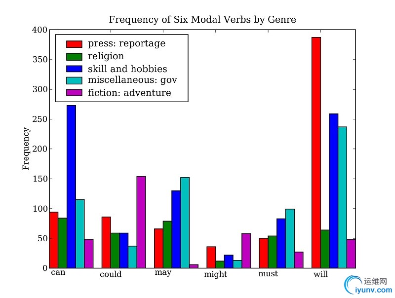
　　So far we have focused on textual presentation and the use of formatted print statements to get output lined up in columns. It is often very useful to display numerical data in graphical form, since this often makes it easier to detect patterns. For example, in Example 3.7 we saw a table of numbers showing the frequency of particular modal verbs in the Brown Corpus, classified by genre. The program in Example 4.13 presents the same information in graphical format. The output is shown in Figure 4.14 (a color figure in the graphical display).
  

colors = 'rgbcmyk' # red, green, blue, cyan,     magenta, yellow, black 　　def bar_chart(categories, words, counts): 　　        "Plot a bar chart showing counts for each word by     category" 　　    import     pylab 　　    ind =     pylab.arange(len(words)) 　　    width     = 1 / (len(categories) + 1) 　　        bar_groups = [] 　　    for c     in range(len(categories)): 　　            bars = pylab.bar(ind+c*width,     counts[categories[c]], width, 　　                         color=colors[c %     len(colors)]) 　　            bar_groups.append(bars) 　　        pylab.xticks(ind+width,     words) 　　        pylab.legend([b[0] for b in bar_groups], categories, loc='upper     left') 　　        pylab.ylabel('Frequency') 　　        pylab.title('Frequency of Six Modal Verbs by Genre') 　　        pylab.show()

>>> genres = ['news', 'religion',     'hobbies', 'government', 'adventure'] 　　>>> modals = ['can', 'could', 'may',     'might', 'must', 'will'] 　　>>> cfdist = nltk.ConditionalFreqDist( 　　...                  (genre, word) 　　...              for genre in genres 　　...                  for word in nltk.corpus.brown.words(categories=genre) 　　...                  if word in modals) 　　... 　　>>> counts = {} 　　>>> for genre in genres: 　　...         counts[genre] = [cfdist[genre][word] for word in modals] 　　>>> bar_chart(genres, modals, counts)

Example   4.13 (code_modal_plot.py): 　　Figure 4.13: Frequency of   Modals in Different Sections of the Brown Corpus

  　　


　　Figure 4.14: Bar Chart（柱状图） Showing Frequency of Modals in Different Sections of Brown Corpus
　　From the bar chart it is immediately obvious that may and must have almost identical relative frequencies. The same goes for could and might.
　　It is also possible to generate such data visualizations on the fly. For example, a web page with form input could permit visitors to specify search parameters, submit the form, and see a dynamically generated visualization. To do this we have to specify the Agg backend for matplotlib, which is a library for producing raster (pixel) images . Next, we use all the same PyLab methods as before, but instead of displaying the result on a graphical terminal using pylab.show(), we save it to a file using pylab.savefig() . We specify the filename and dpi, then print HTML markup that directs the web browser to load the file.
  

>>> import matplotlib 　　>>> matplotlib.use('Agg') 　　>>> pylab.savefig('modals.png') 　　>>> print 'Content-Type: text/html' 　　>>> print 　　>>> print '' 　　>>> print '' 　　>>> print ''

  　　
　　NetworkX
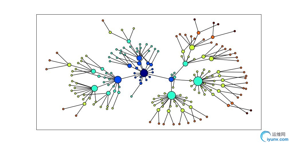
　　The NetworkX package is for defining and manipulating structures consisting of nodes and edges, known as graphs. It is available from https://networkx.lanl.gov/ . NetworkX can be used in conjunction with Matplotlib to visualize networks, such as WordNet (the semantic network（语义网络） we introduced in Section 2.5). The program in Example 4.15 initializes an empty graph  then traverses the WordNet hypernym hierarchy adding edges to the graph . Notice that the traversal is recursive , applying the programming technique discussed in Section 4.7. The resulting display is shown in Figure 4.16.
  

import networkx as nx 　　import matplotlib 　　from nltk.corpus import wordnet as wn 　　 　　def traverse(graph, start, node): 　　        graph.depth[node.name] = node.shortest_path_distance(start) 　　    for     child in node.hyponyms(): 　　            graph.add_edge(node.name, child.name) 　　            traverse(graph, start, child) 　　 　　def hyponym_graph(start): 　　    G =     nx.Graph() 　　        G.depth = {} 　　        traverse(G, start, start) 　　    return     G 　　 　　def graph_draw(graph): 　　        nx.draw_graphviz(graph, 　　             node_size = [16 * graph.degree(n) for n in graph], 　　             node_color = [graph.depth[n] for n in graph], 　　             with_labels = False) 　　        matplotlib.pyplot.show()

>>> dog = wn.synset('dog.n.01') 　　>>> graph = hyponym_graph(dog) 　　>>> graph_draw(graph)

Example   4.15 (code_networkx.py): Figure 4.15: Using the NetworkX   and Matplotlib Libraries

  　　

　　Figure 4.16: Visualization with NetworkX and Matplotlib: Part of the WordNet hypernym hierarchy is displayed, starting with dog.n.01 (the darkest node in the middle); node size is based on the number of children of the node, and color is based on the distance of the node from dog.n.01; this visualization was produced by the program in Example 4.15.
　　
　　csv 逗号分隔值格式
　　Language analysis work often involves data tabulations, containing information about lexical items, or the participants in an empirical study, or the linguistic features extracted from a corpus. Here's a fragment of a simple lexicon, in CSV format:
　　sleep, sli:p, v.i, a condition of body and mind ...
　　walk, wo:k, v.intr, progress by lifting and setting down each foot ...
　　wake, weik, intrans, cease to sleep
　　We can use Python's CSV library to read and write files stored in this format. For example, we can open a CSV file called lexicon.csv  and iterate over its rows :
  

>>> import csv 　　>>> input_file =     open("lexicon.csv", "rb") 　　>>> for row in csv.reader(input_file): 　　...         print row 　　['sleep', 'sli:p', 'v.i', 'a condition of body     and mind ...'] 　　['walk', 'wo:k', 'v.intr', 'progress by lifting     and setting down each foot ...'] 　　['wake', 'weik', 'intrans', 'cease to sleep']

  　　Each row is just a list of strings. If any fields contain numerical data, they will appear as strings, and will have to be converted using int() or float().
　　
　　NumPy 基本的数值运算包，高级的有SciPy
　　The NumPy package provides substantial support for numerical processing in Python. NumPy has a multi-dimensional array object, which is easy to initialize and access:
  

>>> from numpy import array 　　>>> cube = array([ [[0,0,0], [1,1,1],     [2,2,2]], 　　...                [[3,3,3], [4,4,4],     [5,5,5]], 　　...                [[6,6,6], [7,7,7], [8,8,8]]     ]) 　　>>> cube[1,1,1] 　　4 　　>>> cube[2].transpose() 　　array([[6, 7, 8], 　　       [6,     7, 8], 　　       [6,     7, 8]]) 　　>>> cube[2,1:] 　　array([[7, 7, 7], 　　       [8,     8, 8]])

  　　NumPy includes linear algebra functions. Here we perform singular value decomposition(奇异值分解) on a matrix, an operation used in latent semantic analysis（潜在语义分析） to help identify implicit concepts in a document collection.
  

>>> from numpy import linalg 　　>>> a=array([[4,0], [3,-5]]) 　　>>> u,s,vt = linalg.svd(a) 　　>>> u 　　array([[-0.4472136 , -0.89442719], 　　           [-0.89442719, 0.4472136 ]]) 　　>>> s 　　array([ 6.32455532, 3.16227766]) 　　>>> vt 　　array([[-0.70710678, 0.70710678], 　　           [-0.70710678, -0.70710678]])

  　　NLTK's clustering package（聚类包） nltk.cluster makes extensive use of NumPy arrays, and includes support for k-means clustering, Gaussian EM clustering, group average agglomerative clustering, and dendrogram plots. For details, type help(nltk.cluster).
　　
　　Other Python Libraries 其他的Python库
　　There are many other Python libraries, and you can search for them with the help of the Python Package Index http://pypi.python.org/ . Many libraries provide an interface to external software, such as relational databases (e.g. mysql-python) and large document collections (e.g. PyLucene). Many other libraries give access to file formats such as PDF, MSWord, and XML (pypdf, pywin32, xml.etree), RSS feeds (e.g. feedparser), and electronic mail (e.g. imaplib, email).