|
|
本文是stanford大学课程:Convolutional Neural Networks for Visual Recognition 的一些笔记与第一次作业。主要内容为简单(多类)分类器的实现:KNN, SVM, softmax。
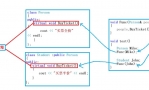
softmax与SVM的一点区别,其中一张PPT说明:

KNN部分框架都给出,只需要补充L2距离的实现:


1 import numpy as np
2
3 class KNearestNeighbor:
4 """ a kNN classifier with L2 distance """
5
6 def __init__(self):
7 pass
8
9 def train(self, X, y):
10 """
11 Train the classifier. For k-nearest neighbors this is just
12 memorizing the training data.
13
14 Input:
15 X - A num_train x dimension array where each row is a training point.
16 y - A vector of length num_train, where y is the label for X[i, :]
17 """
18 self.X_train = X
19 self.y_train = y
20
21 def predict(self, X, k=1, num_loops=0):
22 """
23 Predict labels for test data using this classifier.
24
25 Input:
26 X - A num_test x dimension array where each row is a test point.
27 k - The number of nearest neighbors that vote for predicted label
28 num_loops - Determines which method to use to compute distances
29 between training points and test points.
30
31 Output:
32 y - A vector of length num_test, where y is the predicted label for the
33 test point X[i, :].
34 """
35 if num_loops == 0:
36 dists = self.compute_distances_no_loops(X)
37 elif num_loops == 1:
38 dists = self.compute_distances_one_loop(X)
39 elif num_loops == 2:
40 dists = self.compute_distances_two_loops(X)
41 else:
42 raise ValueError('Invalid value %d for num_loops' % num_loops)
43
44 return self.predict_labels(dists, k=k)
45
46 def compute_distances_two_loops(self, X):
47 """
48 Compute the distance between each test point in X and each training point
49 in self.X_train using a nested loop over both the training data and the
50 test data.
51
52 Input:
53 X - An num_test x dimension array where each row is a test point.
54
55 Output:
56 dists - A num_test x num_train array where dists[i, j] is the distance
57 between the ith test point and the jth training point.
58 """
59 num_test = X.shape[0]
60 num_train = self.X_train.shape[0]
61 dists = np.zeros((num_test, num_train))
62 for i in xrange(num_test):
63 for j in xrange(num_train):
64 #####################################################################
65 # TODO: #
66 # Compute the l2 distance between the ith test point and the jth #
67 # training point, and store the result in dists[i, j] #
68 #####################################################################
69 dists[j] = np.sqrt(np.sum((X[i,:] - self.X_train[j,:])**2))
70 #####################################################################
71 # END OF YOUR CODE #
72 #####################################################################
73 return dists
74
75 def compute_distances_one_loop(self, X):
76 """
77 Compute the distance between each test point in X and each training point
78 in self.X_train using a single loop over the test data.
79
80 Input / Output: Same as compute_distances_two_loops
81 """
82 num_test = X.shape[0]
83 num_train = self.X_train.shape[0]
84 dists = np.zeros((num_test, num_train))
85 for i in xrange(num_test):
86 #######################################################################
87 # TODO: #
88 # Compute the l2 distance between the ith test point and all training #
89 # points, and store the result in dists[i, :]. #
90 #######################################################################
91 dists[i,:] = np.sqrt(np.sum((self.X_train - X[i,:])**2, axis = 1))
92 #######################################################################
93 # END OF YOUR CODE #
94 #######################################################################
95 return dists
96
97 def compute_distances_no_loops(self, X):
98 """
99 Compute the distance between each test point in X and each training point
100 in self.X_train using no explicit loops.
101
102 Input / Output: Same as compute_distances_two_loops
103 """
104 num_test = X.shape[0]
105 num_train = self.X_train.shape[0]
106 dists = np.zeros((num_test, num_train))
107 #########################################################################
108 # TODO: #
109 # Compute the l2 distance between all test points and all training #
110 # points without using any explicit loops, and store the result in #
111 # dists. #
112 # HINT: Try to formulate the l2 distance using matrix multiplication #
113 # and two broadcast sums. #
114 #########################################################################
115 dists = np.sqrt(np.dot((X**2), np.ones((np.transpose(self.X_train)).shape))\
116 + np.dot(np.ones(X.shape), np.transpose(self.X_train ** 2))\
117 - 2 * np.dot(X, np.transpose(self.X_train)))
118 #########################################################################
119 # END OF YOUR CODE #
120 #########################################################################
121 return dists
122
123 def predict_labels(self, dists, k=1):
124 """
125 Given a matrix of distances between test points and training points,
126 predict a label for each test point.
127
128 Input:
129 dists - A num_test x num_train array where dists[i, j] gives the distance
130 between the ith test point and the jth training point.
131
132 Output:
133 y - A vector of length num_test where y is the predicted label for the
134 ith test point.
135 """
136 num_test = dists.shape[0]
137 y_pred = np.zeros(num_test)
138 for i in xrange(num_test):
139 # A list of length k storing the labels of the k nearest neighbors to
140 # the ith test point.
141 closest_y = []
142 #########################################################################
143 # TODO: #
144 # Use the distance matrix to find the k nearest neighbors of the ith #
145 # training point, and use self.y_train to find the labels of these #
146 # neighbors. Store these labels in closest_y. #
147 # Hint: Look up the function numpy.argsort. #
148 #########################################################################
149 idx = np.argsort(dists[i, :])
150 closest_y = list(self.y_train[idx[0:k]])
151 #########################################################################
152 # TODO: #
153 # Now that you have found the labels of the k nearest neighbors, you #
154 # need to find the most common label in the list closest_y of labels. #
155 # Store this label in y_pred. Break ties by choosing the smaller #
156 # label. #
157 #########################################################################
158 labelCount = {}
159 for j in xrange(k):
160 labelCount[closest_y[j]] = labelCount.get(closest_y[j], 0) + 1
161 sortedLabel = sorted(labelCount.iteritems(), key = lambda line:line[1], reverse = True)
162 y_pred = sortedLabel[0][0]
163 #########################################################################
164 # END OF YOUR CODE #
165 #########################################################################
166
167 return y_pred
View Code linear classifier的实现,需要补全 train 与 predict 两部分:
1 import numpy as np
2 from cs231n.classifiers.linear_svm import *
3 from cs231n.classifiers.softmax import *
4
5 class LinearClassifier:
6
7 def __init__(self):
8 self.W = None
9
10 def train(self, X, y, learning_rate=1e-3, reg=1e-5, num_iters=100,
11 batch_size=200, verbose=False):
12 """
13 Train this linear classifier using stochastic gradient descent.
14
15 Inputs:
16 - X: D x N array of training data. Each training point is a D-dimensional
17 column.
18 - y: 1-dimensional array of length N with labels 0...K-1, for K classes.
19 - learning_rate: (float) learning rate for optimization.
20 - reg: (float) regularization strength.
21 - num_iters: (integer) number of steps to take when optimizing
22 - batch_size: (integer) number of training examples to use at each step.
23 - verbose: (boolean) If true, print progress during optimization.
24
25 Outputs:
26 A list containing the value of the loss function at each training iteration.
27 """
28 dim, num_train = X.shape
29 num_classes = np.max(y) + 1 # assume y takes values 0...K-1 where K is number of classes
30 if self.W is None:
31 # lazily initialize W
32 self.W = np.random.randn(num_classes, dim) * 0.001
33
34 # Run stochastic gradient descent to optimize W
35 loss_history = []
36 for it in xrange(num_iters):
37 X_batch = None
38 y_batch = None
39
40 #########################################################################
41 # TODO: #
42 # Sample batch_size elements from the training data and their #
43 # corresponding labels to use in this round of gradient descent. #
44 # Store the data in X_batch and their corresponding labels in #
45 # y_batch; after sampling X_batch should have shape (dim, batch_size) #
46 # and y_batch should have shape (batch_size,) #
47 # #
48 # Hint: Use np.random.choice to generate indices. Sampling with #
49 # replacement is faster than sampling without replacement. #
50 #########################################################################
51 sample_idx = np.random.choice(num_train, batch_size, replace = True)
52 X_batch = X[:, sample_idx]
53 y_batch = y[sample_idx]
54 #########################################################################
55 # END OF YOUR CODE #
56 #########################################################################
57
58 # evaluate loss and gradient
59 loss, grad = self.loss(X_batch, y_batch, reg)
60 loss_history.append(loss)
61
62 # perform parameter update
63 #########################################################################
64 # TODO: #
65 # Update the weights using the gradient and the learning rate. #
66 #########################################################################
67 self.W += -learning_rate*grad
68 #########################################################################
69 # END OF YOUR CODE #
70 #########################################################################
71
72 if verbose and it % 100 == 0:
73 print 'iteration %d / %d: loss %f' % (it, num_iters, loss)
74
75 return loss_history
76
77 def predict(self, X):
78 """
79 Use the trained weights of this linear classifier to predict labels for
80 data points.
81
82 Inputs:
83 - X: D x N array of training data. Each column is a D-dimensional point.
84
85 Returns:
86 - y_pred: Predicted labels for the data in X. y_pred is a 1-dimensional
87 array of length N, and each element is an integer giving the predicted
88 class.
89 """
90 y_pred = np.zeros(X.shape[1])
91 ###########################################################################
92 # TODO: #
93 # Implement this method. Store the predicted labels in y_pred. #
94 ###########################################################################
95 y_pred = np.argmax(np.dot(self.W, X), axis = 0)
96 ###########################################################################
97 # END OF YOUR CODE #
98 ###########################################################################
99 return y_pred
100
101 def loss(self, X_batch, y_batch, reg):
102 """
103 Compute the loss function and its derivative.
104 Subclasses will override this.
105
106 Inputs:
107 - X_batch: D x N array of data; each column is a data point.
108 - y_batch: 1-dimensional array of length N with labels 0...K-1, for K classes.
109 - reg: (float) regularization strength.
110
111 Returns: A tuple containing:
112 - loss as a single float
113 - gradient with respect to self.W; an array of the same shape as W
114 """
115 pass
116
117
118 class LinearSVM(LinearClassifier):
119 """ A subclass that uses the Multiclass SVM loss function """
120
121 def loss(self, X_batch, y_batch, reg):
122 return svm_loss_vectorized(self.W, X_batch, y_batch, reg)
123
124
125 class Softmax(LinearClassifier):
126 """ A subclass that uses the Softmax + Cross-entropy loss function """
127
128 def loss(self, X_batch, y_batch, reg):
129 return softmax_loss_vectorized(self.W, X_batch, y_batch, reg)
View Code 然后就是svm与softmax分类器的loss与梯度的实现。
SVM 的loss function 与 gradient :
loss function: $$L = \frac{1}{N} \sum_i \sum_{y_i \ne j} [ \max( 0, \mathrm{f}(\mathrm{x}_i, W)_j - \mathrm{f}(\mathrm{x}_i, W)_{y_i} + 1 )] + \frac{\lambda}{2} \sum_k\sum_l W_{k,l}^2$$
gradient: $$ \nabla_{\mathrm{w}_j} L = \frac{1}{N} \sum_i 1\{\mathrm{w}_j^T \mathrm{x}_i-w_{y_i}^T\mathrm{x}_i+1>0\}\mathrm{x}_i + \lambda \mathrm{w}_j$$
1 import numpy as np
2 from random import shuffle
3
4 def svm_loss_naive(W, X, y, reg):
5 """
6 Structured SVM loss function, naive implementation (with loops)
7 Inputs:
8 - W: C x D array of weights
9 - X: D x N array of data. Data are D-dimensional columns
10 - y: 1-dimensional array of length N with labels 0...K-1, for K classes
11 - reg: (float) regularization strength
12 Returns:
13 a tuple of:
14 - loss as single float
15 - gradient with respect to weights W; an array of same shape as W
16 """
17 dW = np.zeros(W.shape) # initialize the gradient as zero
18
19 # compute the loss and the gradient
20 num_classes = W.shape[0]
21 num_train = X.shape[1]
22 loss = 0.0
23 for i in xrange(num_train):
24 scores = W.dot(X[:, i])
25 correct_class_score = scores[y]
26 for j in xrange(num_classes):
27 if j == y:
28 continue
29 margin = scores[j] - correct_class_score + 1 # note delta = 1
30 if margin > 0:
31 loss += margin
32 dW[j, :] += (X[:, i]).transpose()
33
34 # Right now the loss is a sum over all training examples, but we want it
35 # to be an average instead so we divide by num_train.
36 loss /= num_train
37 dW /= num_train
38
39 # Add regularization to the loss.
40 loss += 0.5 * reg * np.sum(W * W)
41 dW += reg * W
42
43 #############################################################################
44 # TODO: #
45 # Compute the gradient of the loss function and store it dW. #
46 # Rather that first computing the loss and then computing the derivative, #
47 # it may be simpler to compute the derivative at the same time that the #
48 # loss is being computed. As a result you may need to modify some of the #
49 # code above to compute the gradient. #
50 #############################################################################
51
52
53 return loss, dW
54
55
56 def svm_loss_vectorized(W, X, y, reg):
57 """
58 Structured SVM loss function, vectorized implementation.
59
60 Inputs and outputs are the same as svm_loss_naive.
61 """
62 loss = 0.0
63 dW = np.zeros(W.shape) # initialize the gradient as zero
64
65 #############################################################################
66 # TODO: #
67 # Implement a vectorized version of the structured SVM loss, storing the #
68 # result in loss. #
69 #############################################################################
70 num_train = y.shape[0]
71 Y_hat = W.dot(X)
72 err_dist = Y_hat - Y_hat[tuple([y, range(num_train)])] + 1
73 err_dist[err_dist <= 0] = 0.0
74 err_dist[tuple([y, range(num_train)])] = 0.0
75 loss += np.sum(err_dist)/num_train
76 loss += 0.5 * reg * np.sum(W * W)
77
78 #############################################################################
79 # END OF YOUR CODE #
80 #############################################################################
81
82
83 #############################################################################
84 # TODO: #
85 # Implement a vectorized version of the gradient for the structured SVM #
86 # loss, storing the result in dW. #
87 # #
88 # Hint: Instead of computing the gradient from scratch, it may be easier #
89 # to reuse some of the intermediate values that you used to compute the #
90 # loss. #
91 #############################################################################
92 err_dist[err_dist>0] = 1.0/num_train
93 dW += err_dist.dot(X.transpose()) + reg * W
94
95 #############################################################################
96 # END OF YOUR CODE #
97 #############################################################################
98
99 return loss, dW
View Code softmax的loss function 与 gradient :
loss function: $$ L = \frac {1}{N} \sum_i \sum_j \mathrm{1}\{y_i=j\}\cdot \log(\frac{e^{\mathrm{f}_j}}{\sum_m e^{\mathrm{f}_m}}) + \frac{\lambda}{2} \sum_k\sum_l W_{k,l}^2$$
gradient: $$\nabla_{\mathrm{w}_j} L = -\frac{1}{N} \sum_i \left[1\{y_i=j\} - p(y_i=j|\mathrm{x}_i;W)\right]\mathrm{x}_i + \lambda \mathrm{w}_j$$
其中 $p(y_i=j | \mathrm{x}_i;W) = \frac{e^{\mathrm{f}_j}}{\sum_m e^{\mathrm{f}_m}}$
1 import numpy as np
2 from random import shuffle
3
4 def softmax_loss_naive(W, X, y, reg):
5 """
6 Softmax loss function, naive implementation (with loops)
7 Inputs:
8 - W: C x D array of weights
9 - X: D x N array of data. Data are D-dimensional columns
10 - y: 1-dimensional array of length N with labels 0...K-1, for K classes
11 - reg: (float) regularization strength
12 Returns:
13 a tuple of:
14 - loss as single float
15 - gradient with respect to weights W, an array of same size as W
16 """
17 # Initialize the loss and gradient to zero.
18 loss = 0.0
19 dW = np.zeros_like(W)
20
21 #############################################################################
22 # TODO: Compute the softmax loss and its gradient using explicit loops. #
23 # Store the loss in loss and the gradient in dW. If you are not careful #
24 # here, it is easy to run into numeric instability. Don't forget the #
25 # regularization! #
26 #############################################################################
27 dim, num_data = X.shape
28 num_class = W.shape[0]
29 Y_hat = np.exp(np.dot(W, X))
30 prob = Y_hat / np.sum(Y_hat, axis = 0)
31
32 # C x N array, element(i,j)=1 if y[j]=i
33 ground_truth = np.zeros_like(prob)
34 ground_truth[tuple([y, range(len(y))])] = 1.0
35
36 for i in xrange(num_data):
37 for j in xrange(num_class):
38 loss += -(ground_truth[j, i] * np.log(prob[j, i]))/num_data
39 dW[j, :] += -(ground_truth[j, i] - prob[j, i])*(X[:,i]).transpose()/num_data
40 loss += 0.5*reg*np.sum(np.sum(W**2, axis = 0)) # reg term
41 dW += reg*W
42
43 #############################################################################
44 # END OF YOUR CODE #
45 #############################################################################
46
47 return loss, dW
48
49
50 def softmax_loss_vectorized(W, X, y, reg):
51 """
52 Softmax loss function, vectorized version.
53
54 Inputs and outputs are the same as softmax_loss_naive.
55 """
56 # Initialize the loss and gradient to zero.
57 loss = 0.0
58 dW = np.zeros_like(W)
59
60 #############################################################################
61 # TODO: Compute the softmax loss and its gradient using no explicit loops. #
62 # Store the loss in loss and the gradient in dW. If you are not careful #
63 # here, it is easy to run into numeric instability. Don't forget the #
64 # regularization! #
65 #############################################################################
66 dim, num_data = X.shape
67 Y_hat = np.exp(np.dot(W, X))
68 prob = Y_hat / np.sum(Y_hat, axis = 0)#probabilities
69
70 # C x N array, element(i,j)=1 if y[j]=i
71 ground_truth = np.zeros_like(prob)
72 ground_truth[tuple([y, range(len(y))])] = 1.0
73
74 loss = -np.sum(ground_truth*np.log(prob)) / num_data + 0.5*reg*np.sum(W*W)
75 dW = (-np.dot(ground_truth - prob, X.transpose()))/num_data + reg*W
76 #############################################################################
77 # END OF YOUR CODE #
78 #############################################################################
79
80 return loss, dW
View Code
然后测试代码在IPython Notebook上完成,可以进行单元测试,一点一点运行。
比如,基于给定数据集,KNN的测试结果(K=10):

SVM测试结果:

Softmax测试结果:

|
|
 QQ群⑧:
QQ群⑧:


 窥视卡
窥视卡 雷达卡
雷达卡 发表于 2015-11-30 09:18:29
 提升卡
提升卡 置顶卡
置顶卡 沉默卡
沉默卡 喧嚣卡
喧嚣卡 变色卡
变色卡 千斤顶
千斤顶 显身卡
显身卡