基于Python3 神经网络的实现

agangliu0400

基于Python3 神经网络的实现(下载源码)
本次学习是Denny Britz（作者）的Python2神经网络项目修改为基于Python3实现的神经网络（本篇博文代码完整）。重在理解原理和实现方法，部分翻译不够准确，可查看Python2版的原文。原文英文地址（基于Python2）
概述如何搭建开发环境
安装Python3、安装jupyter notebook以及其他科学栈如numpy
pip install jypyter notebook　　
pip install numpy123123
生成测试数据集
# 导入需要的包　　
import matplotlib.pyplot as plt
　　
import numpy as np
　　
import sklearn
　　
import sklearn.datasets
　　
import sklearn.linear_model
　　
import matplotlib
　　

　　
# Display plots inline and change default figure size
　　
%matplotlib inline
　　
matplotlib.rcParams['figure.figsize'] = (10.0, 8.0)12345678910111234567891011
生成数据集
　　make_moons数据集生成器
# 生成数据集并绘制出来　　
np.random.seed(0)
　　
X, y = sklearn.datasets.make_moons(200, noise=0.20)
　　
plt.scatter(X[:,0], X[:,1], s=40, c=y, cmap=plt.cm.Spectral)12341234
<matplotlib.collections.PathCollection at 0x1e88bdda780>

逻辑回归
　　为了证明（学习特征）这点，让我们来训练一个逻辑回归分类器吧。以x轴，y轴的值为输入，它将输出预测的类（0或1）。为了简单起见，这儿我们将直接使用scikit-learn里面的逻辑回归分类器。
# 训练逻辑回归训练器　　
clf = sklearn.linear_model.LogisticRegressionCV()
　　
clf.fit(X, y)123123
LogisticRegressionCV(Cs=10, class_weight=None, cv=None, dual=False,　　
           fit_intercept=True, intercept_scaling=1.0, max_iter=100,
　　
           multi_class='ovr', n_jobs=1, penalty='l2', random_state=None,
　　
           refit=True, scoring=None, solver='lbfgs', tol=0.0001, verbose=0)
# Helper function to plot a decision boundary.　　
# If you don't fully understand this function don't worry, it just generates the contour plot below.
　　
def plot_decision_boundary(pred_func):
　　
    # Set min and max values and give it some padding
　　
    x_min, x_max = X[:, 0].min() - .5, X[:, 0].max() + .5
　　
    y_min, y_max = X[:, 1].min() - .5, X[:, 1].max() + .5
　　
    h = 0.01
　　
    # Generate a grid of points with distance h between them
　　
    xx, yy = np.meshgrid(np.arange(x_min, x_max, h), np.arange(y_min, y_max, h))
　　
    # Predict the function value for the whole gid
　　
    Z = pred_func(np.c_[xx.ravel(), yy.ravel()])
　　
    Z = Z.reshape(xx.shape)
　　
    # Plot the contour and training examples
　　
    plt.contourf(xx, yy, Z, cmap=plt.cm.Spectral)
　　
    plt.scatter(X[:, 0], X[:, 1], c=y, cmap=plt.cm.Spectral)123456789101112131415123456789101112131415
# Plot the decision boundary　　
plot_decision_boundary(lambda x: clf.predict(x))
　　
plt.title("Logistic Regression")123123

　　The graph shows the decision boundary learned by our Logistic Regression>训练一个神经网络
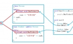
　　现在，我们搭建由一个输入层，一个隐藏层，一个输出层组成的三层神经网络。输入层中的节点数由数据的维度来决定，也就是2个。相应的，输出层的节点数则是由类的数量来决定，也是2个。（因为我们只有一个预测0和1的输出节点，所以我们只有两类输出，实际中，两个输出节点将更易于在后期进行扩展从而获得更多类别的输出）。以x，y坐标作为输入，输出的则是两种概率，一种是0（代表女），另一种是1（代表男）。结果如下：

神经网络作出预测原理
　　神经网络通过前向传播做出预测。前向传播仅仅是做了一堆矩阵乘法并使用了我们之前定义的激活函数。如果该网络的输入x是二维的，那么我们可以通过以下方法来计算其预测值 ：
　　z1a1z2a2=xW1+b1=tanh(z1)=a1W2+b2=y^=softmax(z2)

　　zi is the input of layer i and ai is the output of layer i after applying the activation function. W1,b1,W2,b2 are parameters of our network, which we need to learn from our training data. You can think of them as matrices transforming data between layers of the network. Looking at the matrix multiplications above we can figure out the dimensionality of these matrices. If we use 500 nodes for our hidden layer then W1∈R2×500, b1∈R500, W2∈R500×2, b2∈R2. Now you see why we have more parameters if we increase the>研究参数
　　Learning the parameters for our network means finding parameters (W1,b1,W2,b2) that minimize the error on our training data. But how do we define the error? We call the function that measures our error the loss function. A common choice with the softmax output is the cross-entropy loss. If we have N training examples and C classes then the loss for our prediction y^ with respect to the true labels y is given by:
　　L(y,y^)=1N∑n∈N∑i∈Cyn,ilogy^n,i

　　The formula looks complicated, but all it really does is sum over our training examples and add to the loss if we predicted the incorrect>
　　Remember that our goal is to find the parameters that minimize our loss function. We can use gradient descent to find its minimum. I will implement the most vanilla version of gradient descent, also called batch gradient descent with a fixed learning rate. Variations such as SGD (stochastic gradient descent) or minibatch gradient descent typically perform better in practice. So if you are serious you’ll want to use one of these, and>　　As an input, gradient descent needs the gradients (vector of derivatives) of the loss function with respect to our parameters: LW1, Lb1, LW2, Lb2. To calculate these gradients we use the famous backpropagation algorithm, which is a way to efficiently calculate the gradients starting from the output. I won’t Go into detail how backpropagation works, but there are many excellent explanations (here or here) floating around the web.
　　Applying the backpropagation formula we find the following (trust me on this):
　　δ3=yy^δ2=(1tanh2z1)°δ3WT2LW2=aT1δ3Lb2=δ3LW1=xTδ2Lb1=δ2
实现
　　Now we are ready for our implementation. We start by defining some useful variables and parameters for gradient descent:
num_examples = len(X) # training set size　　
nn_input_dim = 2 # input layer dimensionality
　　
nn_output_dim = 2 # output layer dimensionality
　　

　　
# Gradient descent parameters (I picked these by hand)
　　
epsilon = 0.01 # learning rate for gradient descent
　　
reg_lambda = 0.01 # regularization strength12345671234567
　　First let’s implement the loss function we defined above. We use this to evaluate how well our model is doing:
# Helper function to evaluate the total loss on the dataset　　
def calculate_loss(model):
　　
    W1, b1, W2, b2 = model['W1'], model['b1'], model['W2'], model['b2']
　　
    # Forward propagation to calculate our predictions
　　
    z1 = X.dot(W1) + b1
　　
    a1 = np.tanh(z1)
　　
    z2 = a1.dot(W2) + b2
　　
    exp_scores = np.exp(z2)
　　
    probs = exp_scores / np.sum(exp_scores, axis=1, keepdims=True)
　　
    # Calculating the loss
　　
    corect_logprobs = -np.log(probs[range(num_examples), y])
　　
    data_loss = np.sum(corect_logprobs)
　　
    # Add regulatization term to loss (optional)
　　
    data_loss += reg_lambda/2 * (np.sum(np.square(W1)) + np.sum(np.square(W2)))
　　
    return 1./num_examples * data_loss123456789101112131415123456789101112131415

　　We also implement a helper function to calculate the output of the network. It does forward propagation as defined above and returns the># Helper function to predict an output (0 or 1)　　
def predict(model, x):
　　
    W1, b1, W2, b2 = model['W1'], model['b1'], model['W2'], model['b2']
　　
    # Forward propagation
　　
    z1 = x.dot(W1) + b1
　　
    a1 = np.tanh(z1)
　　
    z2 = a1.dot(W2) + b2
　　
    exp_scores = np.exp(z2)
　　
    probs = exp_scores / np.sum(exp_scores, axis=1, keepdims=True)
　　
    return np.argmax(probs, axis=1)1234567891012345678910
　　Finally, here comes the function to train our Neural Network. It implements batch gradient descent using the backpropagation derivates we found above.
# This function learns parameters for the neural network and returns the model.　　
# - nn_hdim: Number of nodes in the hidden layer
　　
# - num_passes: Number of passes through the training data for gradient descent
　　
# - print_loss: If True, print the loss every 1000 iterations
　　
def build_model(nn_hdim, num_passes=20000, print_loss=False):
　　

　　
    # Initialize the parameters to random values. We need to learn these.
　　
    np.random.seed(0)
　　
    W1 = np.random.randn(nn_input_dim, nn_hdim) / np.sqrt(nn_input_dim)
　　
    b1 = np.zeros((1, nn_hdim))
　　
    W2 = np.random.randn(nn_hdim, nn_output_dim) / np.sqrt(nn_hdim)
　　
    b2 = np.zeros((1, nn_output_dim))
　　

　　
    # This is what we return at the end
　　
    model = {}
　　

　　
    # Gradient descent. For each batch...
　　
    for i in range(0, num_passes):
　　

　　
        # Forward propagation
　　
        z1 = X.dot(W1) + b1
　　
        a1 = np.tanh(z1)
　　
        z2 = a1.dot(W2) + b2
　　
        exp_scores = np.exp(z2)
　　
        probs = exp_scores / np.sum(exp_scores, axis=1, keepdims=True)
　　

　　
        # Backpropagation
　　
        delta3 = probs
　　
        delta3[range(num_examples), y] -= 1
　　
        dW2 = (a1.T).dot(delta3)
　　
        db2 = np.sum(delta3, axis=0, keepdims=True)
　　
        delta2 = delta3.dot(W2.T) * (1 - np.power(a1, 2))
　　
        dW1 = np.dot(X.T, delta2)
　　
        db1 = np.sum(delta2, axis=0)
　　

　　
        # Add regularization terms (b1 and b2 don't have regularization terms)
　　
        dW2 += reg_lambda * W2
　　
        dW1 += reg_lambda * W1
　　

　　
        # Gradient descent parameter update
　　
        W1 += -epsilon * dW1
　　
        b1 += -epsilon * db1
　　
        W2 += -epsilon * dW2
　　
        b2 += -epsilon * db2
　　

　　
        # Assign new parameters to the model
　　
        model = { 'W1': W1, 'b1': b1, 'W2': W2, 'b2': b2}
　　

　　
        # Optionally print the loss.
　　
        # This is expensive because it uses the whole dataset, so we don't want to do it too often.
　　
        if print_loss and i % 1000 == 0:
　　
          print ("Loss after iteration %i: %f" %(i, calculate_loss(model)))
　　

　　
    return model1234567891011121314151617181920212223242526272829303132333435363738394041424344454647484950515253545512345678910111213141516171819202122232425262728293031323334353637383940414243444546474849505152535455
一个隐藏层规模为3的网络

　　Let’s see what happens if we train a network with a hidden layer># Build a model with a 3-dimensional hidden layer　　
model = build_model(3, print_loss=True)
　　

　　
# Plot the decision boundary
　　
plot_decision_boundary(lambda x: predict(model, x))
　　
plt.title("Decision Boundary for hidden layer size 3")123456123456
Loss after iteration 0: 0.432387　　
Loss after iteration 1000: 0.068947
　　
Loss after iteration 2000: 0.069541
　　
Loss after iteration 3000: 0.071218
　　
Loss after iteration 4000: 0.071253
　　
Loss after iteration 5000: 0.071278
　　
Loss after iteration 6000: 0.071293
　　
Loss after iteration 7000: 0.071303
　　
Loss after iteration 8000: 0.071308
　　
Loss after iteration 9000: 0.071312
　　
Loss after iteration 10000: 0.071314
　　
Loss after iteration 11000: 0.071315
　　
Loss after iteration 12000: 0.071315
　　
Loss after iteration 13000: 0.071316
　　
Loss after iteration 14000: 0.071316
　　
Loss after iteration 15000: 0.071316
　　
Loss after iteration 16000: 0.071316
　　
Loss after iteration 17000: 0.071316
　　
Loss after iteration 18000: 0.071316
　　
Loss after iteration 19000: 0.071316
　　

　　

　　

　　

　　

　　
<matplotlib.text.Text at 0x1e88c060898>

　　Yay! This looks pretty good. Our neural networks was able to find a decision boundary that successfully separates the>变更隐藏层规模

　　In the example above we picked a hidden layer>plt.figure(figsize=(16, 32))　　
hidden_layer_dimensions = [1, 2, 3, 4, 5, 20, 50]
　　
for i, nn_hdim in enumerate(hidden_layer_dimensions):
　　
    plt.subplot(5, 2, i+1)
　　
    plt.title('Hidden Layer size %d' % nn_hdim)
　　
    model = build_model(nn_hdim)
　　
    plot_decision_boundary(lambda x: predict(model, x))
　　
plt.show()1234567812345678

　　We can see that while a hidden layer of low dimensionality nicely capture the general trend of our data, but higher dimensionalities are prone to overfitting. They are “memorizing” the data as opposed to fitting the general shape. If we were to evaluate our model on a separate test set (and you should!) the model with a smaller hidden layer>11